Quantifying uncertainty in (differential) rhythmicity • limorhyde2

Introduction

Here we show how to use limorhyde2 to quantify uncertainty in rhythmicity and differential rhythmicity. This step is not essential and can be computationally expensive, but can provide additional information. As limorhyde2 is a Bayesian approach focused on effect sizes rather than statistical significance, quantifying uncertainty relies on the concepts of posterior probability and credible intervals.

The data are based on liver samples from wild-type and Rev-erb double-knockout mice (Cho et al. 2012 and GSE34018).

Load packages

library('cowplot')
library('data.table')
library('ggplot2')
library('limorhyde2')
library('qs')

doParallel::registerDoParallel()
theme_set(theme_bw())

Load the data

The expression data are in a matrix with one row per gene and one column per sample. The metadata are in a table with one row per sample. To save time and space, the expression data include only a subset of genes.

y = qread(system.file('extdata', 'GSE34018_data.qs', package = 'limorhyde2'))
y[1:5, 1:5]
#>       GSM840516 GSM840517 GSM840518 GSM840519 GSM840520
#> 12686 11.962830 11.923338 11.098814 10.958933  9.256413
#> 13170  8.989743  9.132606 12.381036 12.441759 14.766070
#> 26897 11.515292 11.625519 10.579969 10.601969 11.096489
#> 11287  7.985859  7.930935  7.674688  7.899531  7.768563
#> 11731  8.481372  8.114623  8.058194  8.144267  8.152959

metadata = qread(system.file('extdata', 'GSE34018_metadata.qs', package = 'limorhyde2'))
metadata
#>        sample      cond time
#>  1: GSM840516 wild-type    0
#>  2: GSM840517 wild-type    0
#>  3: GSM840518 wild-type    4
#>  4: GSM840519 wild-type    4
#>  5: GSM840520 wild-type    8
#>  6: GSM840521 wild-type    8
#>  7: GSM840522 wild-type   12
#>  8: GSM840523 wild-type   12
#>  9: GSM840524 wild-type   16
#> 10: GSM840525 wild-type   16
#> 11: GSM840526 wild-type   20
#> 12: GSM840527 wild-type   20
#> 13: GSM840504  knockout    0
#> 14: GSM840505  knockout    0
#> 15: GSM840506  knockout    4
#> 16: GSM840507  knockout    4
#> 17: GSM840508  knockout    8
#> 18: GSM840509  knockout    8
#> 19: GSM840510  knockout   12
#> 20: GSM840511  knockout   12
#> 21: GSM840512  knockout   16
#> 22: GSM840513  knockout   16
#> 23: GSM840514  knockout   20
#> 24: GSM840515  knockout   20
#>        sample      cond time

Fit linear models and compute posterior fits

Because the samples were acquired at relatively low temporal resolution (every 4 h), we use three knots instead of the default four, which reduces the flexibility of the spline curves. We specify condColname so getModelFit() knows to fit a differential rhythmicity model.

fit = getModelFit(y, metadata, nKnots = 3L, condColname = 'cond')
fit = getPosteriorFit(fit)
#>  - Computing 100 x 109 likelihood matrix.
#>  - Likelihood calculations took 0.09 seconds.
#>  - Fitting model with 109 mixture components.
#>  - Model fitting took 0.02 seconds.
#>  - Computing posterior matrices.
#>  - Computation allocated took 0.02 seconds.

Draw samples from the posterior fits

The posterior fits consist of not just a single set of model coefficients (the posterior means), but distributions of model coefficients. Sampling from these distributions is the first step to quantifying uncertainty in the fits. Here we generate 50 posterior samples, although an actual analysis would require more to accurately estimate the credible intervals.

fit = getPosteriorSamples(fit, nPosteriorSamples = 50L)

Get fitted time-courses

We can use the posterior samples to quantify uncertainty in the expected measurements, i.e., the fitted curves, by specifying the fitType argument. Here we focus on three genes.

genes = data.table(id = c('13170', '12686', '26897'),
                   symbol = c('Dbp', 'Elovl3', 'Acot1'))
times = seq(0, 24, 0.5)

measFitSamps = getExpectedMeas(
  fit, times = times, fitType = 'posterior_samples', features = genes$id)
measFitSamps[genes, symbol := i.symbol, on = .(feature = id)]
print(measFitSamps, nrows = 10L)
#>        time      cond feature     value posterior_sample symbol
#>     1:    0 wild-type   13170  9.389048                1    Dbp
#>     2:    0 wild-type   12686 11.879609                1 Elovl3
#>     3:    0 wild-type   26897 11.516696                1  Acot1
#>     4:    0  knockout   13170 12.149865                1    Dbp
#>     5:    0  knockout   12686 10.193404                1 Elovl3
#>    ---                                                         
#> 14696:   24 wild-type   12686 11.846712               50 Elovl3
#> 14697:   24 wild-type   26897 11.494776               50  Acot1
#> 14698:   24  knockout   13170 11.940549               50    Dbp
#> 14699:   24  knockout   12686 10.013645               50 Elovl3
#> 14700:   24  knockout   26897  9.140671               50  Acot1

Given the expected measurements from the posterior samples, we can compute the lower and upper bounds of the credible interval for each combination of feature, condition, and time-point. By default, getExpectedMeasIntervals() calculates the 90% equal-tailed interval.

measFitInts = getExpectedMeasIntervals(measFitSamps)
print(measFitInts, nrows = 10L)
#>      time      cond feature symbol     lower     upper
#>   1:    0 wild-type   13170    Dbp  9.312920  9.545719
#>   2:    0 wild-type   12686 Elovl3 11.742144 11.956802
#>   3:    0 wild-type   26897  Acot1 11.451277 11.683526
#>   4:    0  knockout   13170    Dbp 11.989281 12.456412
#>   5:    0  knockout   12686 Elovl3  9.896537 10.239946
#>  ---                                                  
#> 290:   24 wild-type   12686 Elovl3 11.742144 11.956802
#> 291:   24 wild-type   26897  Acot1 11.451277 11.683526
#> 292:   24  knockout   13170    Dbp 11.989281 12.456412
#> 293:   24  knockout   12686 Elovl3  9.896537 10.239946
#> 294:   24  knockout   26897  Acot1  9.094299  9.510977

It’s always a good idea to also calculate the posterior mean fitted curves.

measFitMean = getExpectedMeas(fit, times = times, features = genes$id)
measFitMean[genes, symbol := i.symbol, on = .(feature = id)]

Now we can plot the results. In the first row, each curve corresponds to a posterior sample. In the second row, the ribbons indicate the credible intervals.

timeBreaks = seq(0, 24, 4)
pal = 'Dark2'

p1 = ggplot(measFitSamps) +
  facet_wrap(vars(symbol), scales = 'fixed', nrow = 1) +
  geom_line(aes(x = time, y = value, color = cond,
                group = interaction(cond, posterior_sample)), alpha = 0.2) +
  labs(x = 'Circadian time (h)', y = 'Expression (norm.)', color = 'Condition') +
  scale_x_continuous(breaks = timeBreaks) +
  scale_color_brewer(palette = pal) +
  theme(legend.position = 'none')

p2 = ggplot() +
  facet_wrap(vars(symbol), scales = 'fixed', nrow = 1) +
  geom_ribbon(aes(x = time, ymin = lower, ymax = upper, fill = cond),
              alpha = 0.3, data = measFitInts) +
  geom_line(aes(x = time, y = value, color = cond), data = measFitMean) +
  labs(x = 'Circadian time (h)', y = 'Expression (norm.)', color = 'Condition',
       fill = 'Condition') +
  scale_x_continuous(breaks = timeBreaks) +
  scale_fill_brewer(palette = pal) +
  scale_color_brewer(palette = pal) +
  theme(legend.position = 'bottom')

plot_grid(p1, p2, ncol = 1, rel_heights = c(1, 1.25))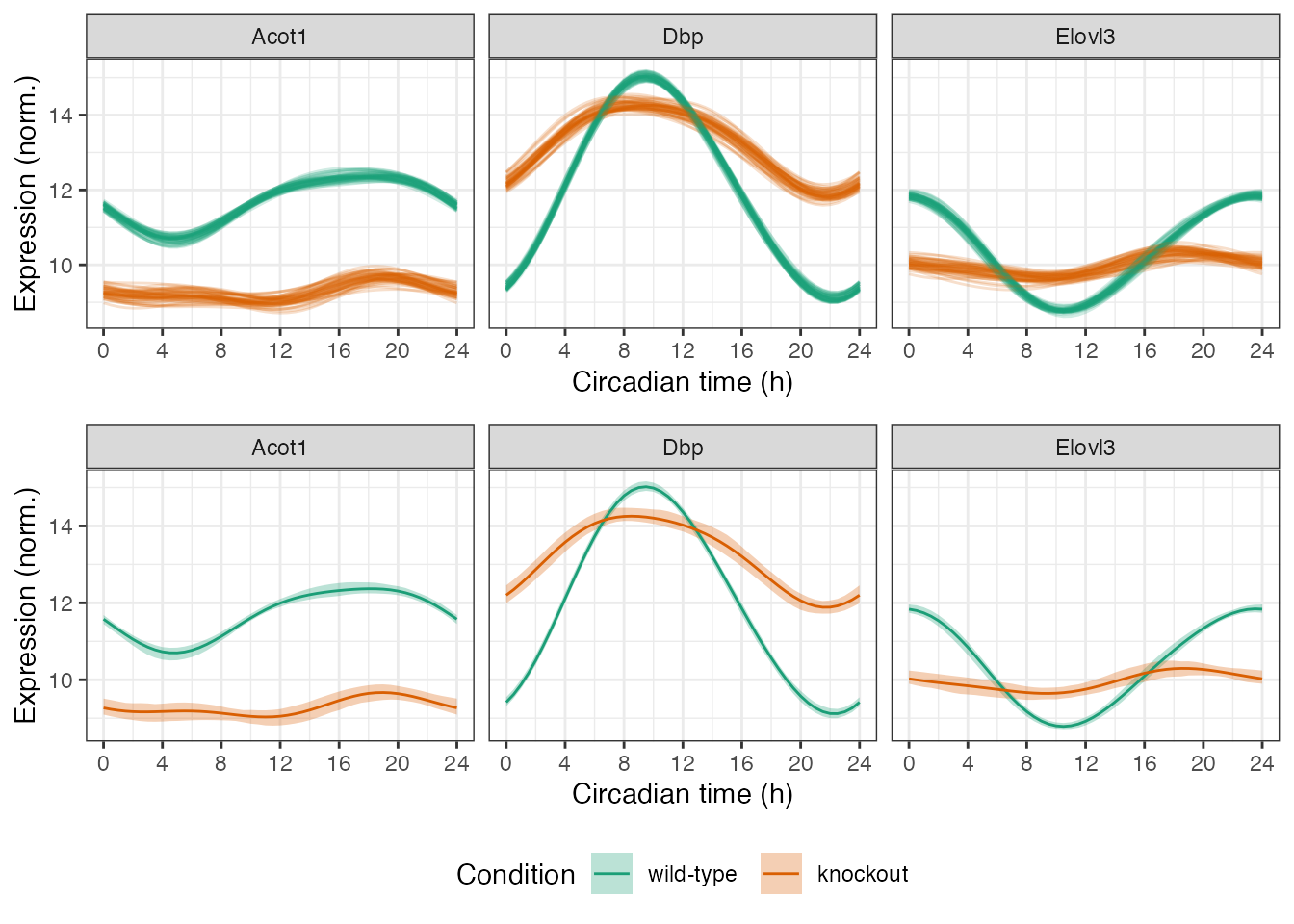

Get rhythmic and differentially rhythmic statistics

We can also use the posterior samples to quantify uncertainty in the statistics, again by specifying the fitType argument.

rhyStatsSamps = getRhythmStats(fit, features = genes$id, fitType = 'posterior_samples')
diffRhyStatsSamps = getDiffRhythmStats(fit, rhyStatsSamps, levels(metadata$cond))
diffRhyStatsSamps[genes, symbol := i.symbol, on = .(feature = id)]
print(diffRhyStatsSamps, nrows = 10L)
#>      feature posterior_sample diff_mean_value diff_peak_trough_amp diff_rms_amp
#>   1:   13170                1       1.2652094           -3.4104140   -1.1872512
#>   2:   12686                1      -0.4083296           -2.5671171   -0.8933007
#>   3:   26897                1      -2.4146956           -1.1408687   -0.4356361
#>   4:   13170                2       1.1635651           -3.3541973   -1.1754108
#>   5:   12686                2      -0.3386511           -2.5290374   -0.9056453
#>  ---                                                                           
#> 146:   12686               49      -0.3658892           -2.1885185   -0.7711306
#> 147:   26897               49      -2.3018778           -0.5256044   -0.1902584
#> 148:   13170               50       1.2099252           -3.4876188   -1.2057042
#> 149:   12686               50      -0.3533242           -2.0847962   -0.7330213
#> 150:   26897               50      -2.4027325           -0.9094560   -0.3389905
#>      diff_peak_phase diff_trough_phase rms_diff_rhy symbol
#>   1:      -0.3951722        -0.3249089    3.0120583    Dbp
#>   2:      -1.8136085        -0.8240157    2.9171445 Elovl3
#>   3:       2.4227880         7.6804644    1.7716140  Acot1
#>   4:      -0.8279032        -0.6553304    3.1222228    Dbp
#>   5:      -5.3312776        -0.9626241    2.9589698 Elovl3
#>  ---                                                      
#> 146:      -5.3694042        -1.4926285    2.7184486 Elovl3
#> 147:      -0.9409261         4.1293078    0.9590076  Acot1
#> 148:       0.5831223         0.0540993    3.5982780    Dbp
#> 149:      -5.0876901        -1.4325180    2.8308634 Elovl3
#> 150:       0.9645104        -1.9435250    1.2260647  Acot1

In the plots below, each point represents a posterior sample.

p1 = ggplot(diffRhyStatsSamps) +
  facet_wrap(vars(symbol), nrow = 1) +
  geom_point(aes(x = diff_peak_trough_amp, y = diff_mean_value), alpha = 0.2) +
  labs(x = 'Difference in peak-to-trough amplitude (norm.)',
       y = 'Difference in mean value (norm.)')

p2 = ggplot(diffRhyStatsSamps) +
  facet_wrap(vars(symbol), nrow = 1) +
  geom_point(aes(x = diff_peak_trough_amp, y = diff_peak_phase), alpha = 0.2) +
  labs(x = 'Difference in peak-to-trough amplitude (norm.)',
       y = 'Difference in peak phase (h)')

plot_grid(p1, p2, ncol = 1)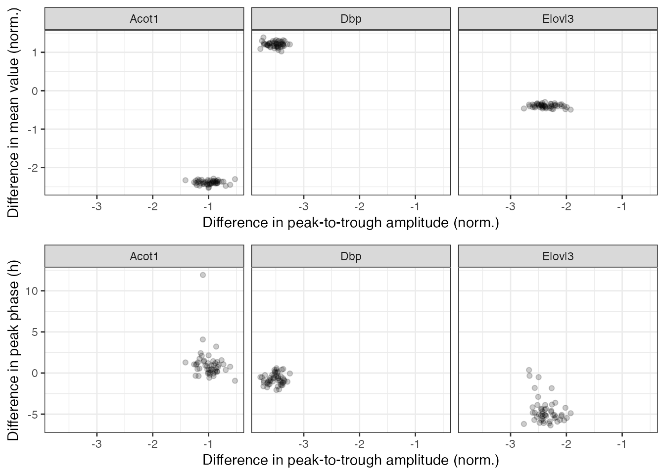

Finally, we can compute credible intervals for the rhythmic and differentially rhythmic statistics. Again, by default these are 90% equal-tailed intervals. Currently getStatsIntervals() does not calculate intervals for phase-based statistics, since phase and phase difference are circular quantities.

rhyStatsInts = getStatsIntervals(rhyStatsSamps)
print(rhyStatsInts, nrows = 10L)
#>          cond feature  statistic      lower      upper
#>  1: wild-type   13170 peak_value 14.9142461 15.1623426
#>  2: wild-type   12686 peak_value 11.7551992 11.9611959
#>  3: wild-type   26897 peak_value 12.2489294 12.5386247
#>  4:  knockout   13170 peak_value 14.1364485 14.4867027
#>  5:  knockout   12686 peak_value 10.1298897 10.5075167
#> ---                                                   
#> 20: wild-type   12686    rms_amp  1.0160493  1.1338332
#> 21: wild-type   26897    rms_amp  0.5069692  0.7253600
#> 22:  knockout   13170    rms_amp  0.7402332  0.9774765
#> 23:  knockout   12686    rms_amp  0.1561527  0.3623270
#> 24:  knockout   26897    rms_amp  0.1459739  0.3350913

diffRhyStatsInts = getStatsIntervals(diffRhyStatsSamps)
print(diffRhyStatsInts, nrows = 10L)
#>     feature            statistic      lower      upper
#>  1:   13170      diff_mean_value  1.0946908  1.3077532
#>  2:   12686      diff_mean_value -0.4761391 -0.3273693
#>  3:   26897      diff_mean_value -2.4744074 -2.3132504
#>  4:   13170 diff_peak_trough_amp -3.7189186 -3.3477383
#>  5:   12686 diff_peak_trough_amp -2.6358331 -2.0279483
#> ---                                                   
#>  8:   12686         diff_rms_amp -0.9157380 -0.7132926
#>  9:   26897         diff_rms_amp -0.4515353 -0.2527135
#> 10:   13170         rms_diff_rhy  2.9709990  3.7122262
#> 11:   12686         rms_diff_rhy  2.5099833  3.0244154
#> 12:   26897         rms_diff_rhy  1.0219593  1.7844688