Introduction
Here we show how to use limorhyde2 to quantify rhythmicity in data from one condition. The data are based on mouse liver samples from the circadian gene expression atlas in mammals (GSE54650).
Load packages
library('data.table')
library('ggplot2')
library('limorhyde2')
library('qs')

doParallel::registerDoParallel()
theme_set(theme_bw())
Load the data
The expression data are in a matrix with one row per gene and one column per sample. The metadata are in a table with one row per sample. To save time and space, the expression data include only a subset of genes.
y = qread(system.file('extdata', 'GSE54650_liver_data.qs', package = 'limorhyde2'))
y[1:5, 1:5]
#>           GSM1321182 GSM1321183 GSM1321184 GSM1321185 GSM1321186
#> 13088      10.209968  10.503358   9.714828   9.477728  10.134381
#> 13170       7.871989   7.281691   6.946495   6.266409   7.150140
#> 13869       6.851685   7.406234   7.781294   7.924764   8.089538
#> 100009600   5.055931   5.199767   5.121511   5.155912   5.219873
#> 100042372   7.497568   7.537684   7.486390   7.502488   7.771348

metadata = qread(system.file('extdata', 'GSE54650_liver_metadata.qs', package = 'limorhyde2'))
metadata
#>         sample time
#>  1: GSM1321182   18
#>  2: GSM1321183   20
#>  3: GSM1321184   22
#>  4: GSM1321185   24
#>  5: GSM1321186   26
#>  6: GSM1321187   28
#>  7: GSM1321188   30
#>  8: GSM1321189   32
#>  9: GSM1321190   34
#> 10: GSM1321191   36
#> 11: GSM1321192   38
#> 12: GSM1321193   40
#> 13: GSM1321194   42
#> 14: GSM1321195   44
#> 15: GSM1321196   46
#> 16: GSM1321197   48
#> 17: GSM1321198   50
#> 18: GSM1321199   52
#> 19: GSM1321200   54
#> 20: GSM1321201   56
#> 21: GSM1321202   58
#> 22: GSM1321203   60
#> 23: GSM1321204   62
#> 24: GSM1321205   64
#>         sample time
Fit linear models
The first step is to fit a series of linear models based on periodic splines for each genomic feature, in this case each gene, using limma. getModelFit() takes several arguments besides the expression data and metadata, but here we just use the defaults. For example, the data are from one condition, so we leave condColname as NULL. Also, the expression data are from microarrays and already log-transformed, so we leave method as 'trend'.
fit = getModelFit(y, metadata)Get posterior fits
The next step is obtain posterior estimates of the model coefficients using multivariate adaptive shrinkage (mashr), which learns patterns in the data and accounts for noise in the original fits.
fit = getPosteriorFit(fit)
#>  - Computing 100 x 121 likelihood matrix.
#>  - Likelihood calculations took 0.04 seconds.
#>  - Fitting model with 121 mixture components.
#>  - Model fitting took 0.03 seconds.
#>  - Computing posterior matrices.
#>  - Computation allocated took 0.01 seconds.
Get rhythmic statistics
We can now use the posterior fits to compute rhythmic statistics, i.e. properties of the curve, for each gene.
rhyStats = getRhythmStats(fit)We can examine the distributions of the statistics in various ways, such as ranking genes by peak-to-trough amplitude (no p-values necessary) or plotting peak-to-trough amplitude vs. peak phase.
print(rhyStats[order(-peak_trough_amp)], nrows = 10L)
#>      feature peak_phase peak_value trough_phase trough_value peak_trough_amp
#>   1:   13170   8.170707  10.403455    23.098021     6.650460     3.752995586
#>   2:   13088  17.371840  10.412731     9.486070     8.643263     1.769468014
#>   3:   13869   8.533100   8.576158    17.957528     7.189246     1.386911808
#>   4:   17988   2.372999   8.821592    10.767925     7.992012     0.829580649
#>   5:  228775   5.350470   7.055462    21.812359     6.241955     0.813506845
#>  ---
#>  96:   11936  10.936695   5.920143     4.556854     5.913565     0.006578039
#>  97:  384185  14.886061   4.783283    21.873340     4.777192     0.006091303
#>  98:  258976  10.936628   5.030834    17.620287     5.025746     0.005088350
#>  99:  269593   6.379766   7.980898    21.265848     7.976391     0.004507119
#> 100:  723939   7.898734   3.908435    23.696203     3.908292     0.000143048
#>           rms_amp mean_value
#>   1: 1.245311e+00   8.478881
#>   2: 5.832602e-01   9.761782
#>   3: 4.670219e-01   7.853253
#>   4: 2.718335e-01   8.343387
#>   5: 2.510419e-01   6.575353
#>  ---
#>  96: 1.908803e-03   5.917020
#>  97: 1.933979e-03   4.781062
#>  98: 1.554801e-03   5.027786
#>  99: 1.514756e-03   7.978485
#> 100: 4.541182e-05   3.908352

ggplot(rhyStats) +
  geom_point(aes(x = peak_phase, y = peak_trough_amp), alpha = 0.2) +
  xlab('Peak phase (h)') +
  ylab('Peak-to-trough amplitude (norm.)') +
  scale_x_continuous(breaks = seq(0, 24, 4))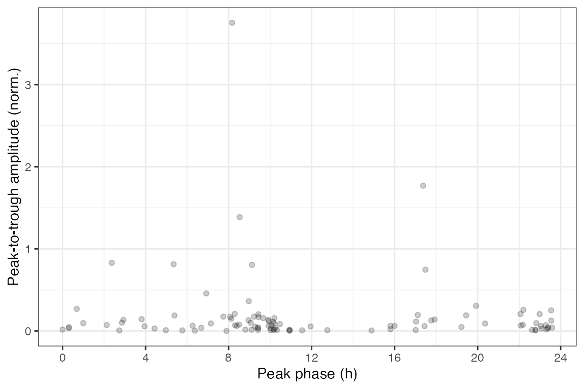
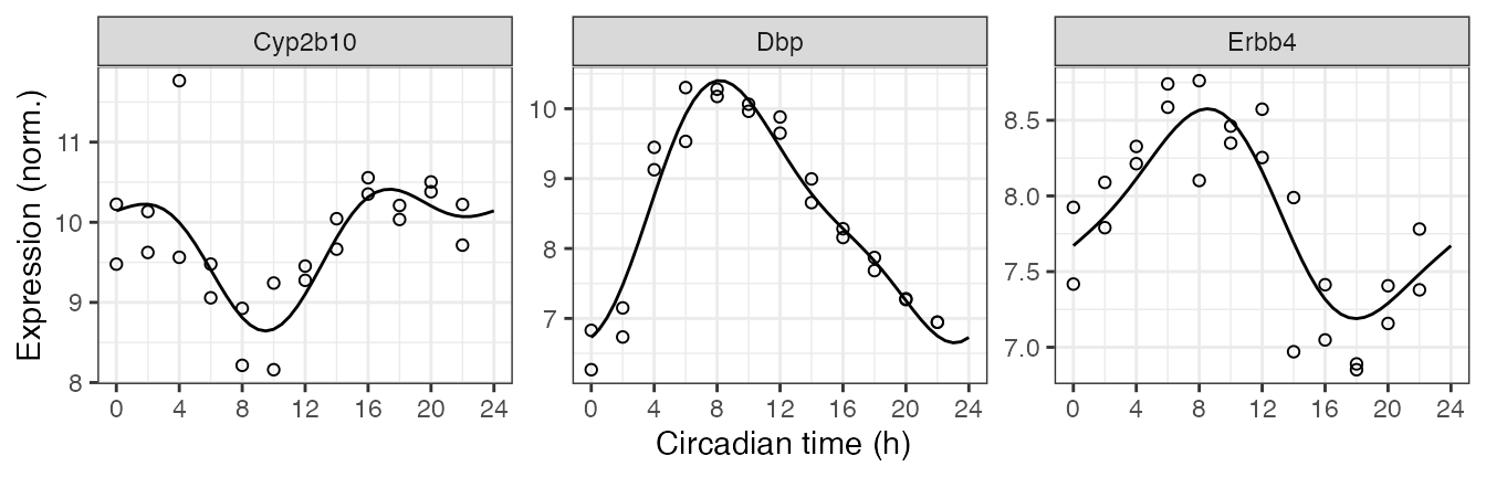
Get observed and fitted time-courses
We can also compute the expected measurements for one or more genes at one or more time-points, which correspond to the fitted curves. Here we plot the posterior fits and observed expression for three of the top rhythmic genes (converting from gene id to gene symbol).
genes = data.table(id = c('13088', '13170', '13869'),
                   symbol = c('Cyp2b10', 'Dbp', 'Erbb4'))

measFit = getExpectedMeas(fit, times = seq(0, 24, 0.5), features = genes$id)
measFit[genes, symbol := i.symbol, on = .(feature = id)]
print(measFit, nrows = 10L)
#>      time feature     value  symbol
#>   1:  0.0   13088 10.142704 Cyp2b10
#>   2:  0.0   13170  6.727867     Dbp
#>   3:  0.0   13869  7.670906   Erbb4
#>   4:  0.5   13088 10.175814 Cyp2b10
#>   5:  0.5   13170  6.842549     Dbp
#>  ---
#> 143: 23.5   13170  6.665309     Dbp
#> 144: 23.5   13869  7.625849   Erbb4
#> 145: 24.0   13088 10.142704 Cyp2b10
#> 146: 24.0   13170  6.727867     Dbp
#> 147: 24.0   13869  7.670906   Erbb4
Next we combine the observed expression data and metadata. The curves show how limorhyde2 is able to fit non-sinusoidal rhythms.
measObs = mergeMeasMeta(y, metadata, features = genes$id)
measObs[genes, symbol := i.symbol, on = .(feature = id)]
print(measObs, nrows = 10L)
#>         sample time feature      meas  symbol
#>  1: GSM1321182   18   13088 10.209968 Cyp2b10
#>  2: GSM1321182   18   13170  7.871989     Dbp
#>  3: GSM1321182   18   13869  6.851685   Erbb4
#>  4: GSM1321183   20   13088 10.503358 Cyp2b10
#>  5: GSM1321183   20   13170  7.281691     Dbp
#> ---
#> 68: GSM1321204   62   13170  8.656560     Dbp
#> 69: GSM1321204   62   13869  6.970524   Erbb4
#> 70: GSM1321205   64   13088 10.352095 Cyp2b10
#> 71: GSM1321205   64   13170  8.157525     Dbp
#> 72: GSM1321205   64   13869  7.048457   Erbb4

ggplot() +
  facet_wrap(vars(symbol), scales = 'free_y', nrow = 1) +
  geom_line(aes(x = time, y = value), data = measFit) +
  geom_point(aes(x = time %% 24, y = meas), shape = 21, size = 1.5,
             data = measObs) +
  labs(x = 'Circadian time (h)', y = 'Expression (norm.)') +
  scale_x_continuous(breaks = seq(0, 24, 4))